 ReelAtlas
Guides
How to read a histogram without guessing
Counts, proportions, density and bin boundaries, illustrated with ten numbers.
On this page
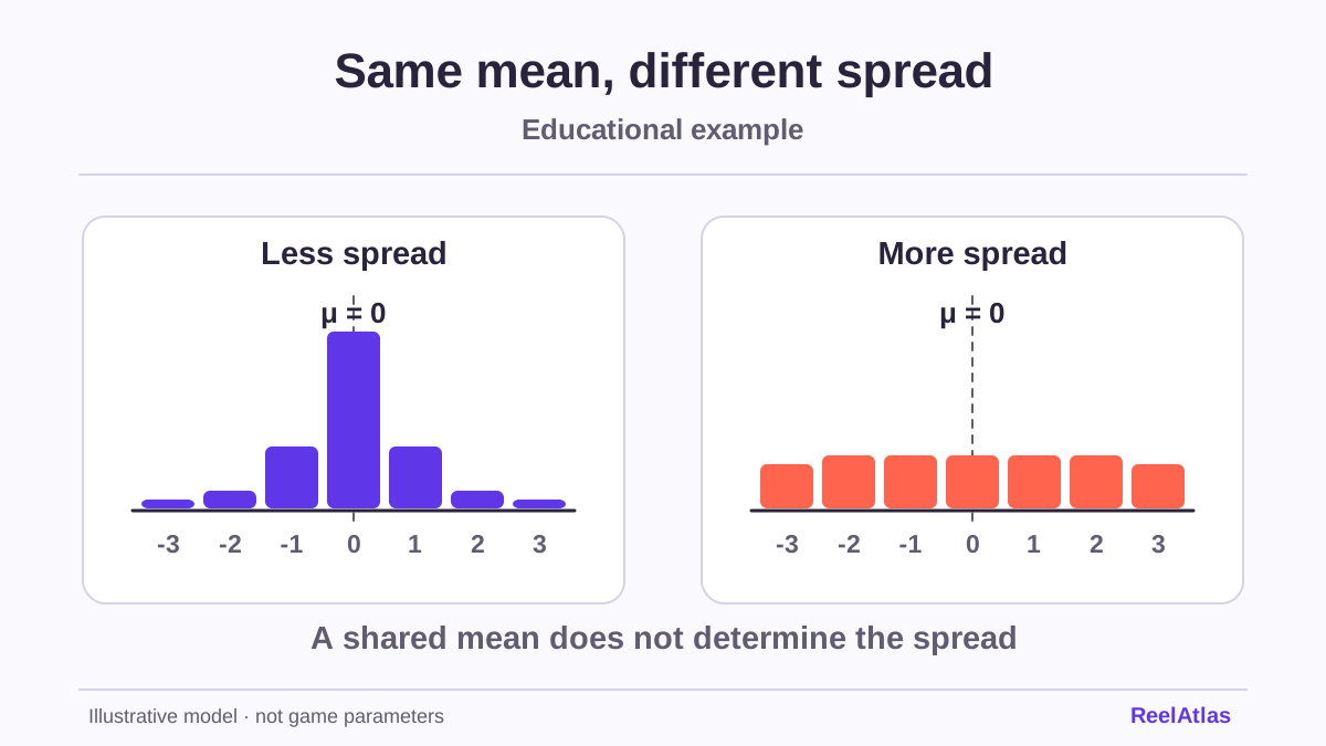
One tall bar can dominate a chart. Before taking it as evidence that large outcomes are frequent, read both axes and check how the data were grouped. A histogram shows how many observations fall into numerical intervals. It leaves their order open.
Build a chart from ten numbers
Take this artificial record of returns: 0, 0, 0, 0, 0.5, 0.5, 1, 2, 4 and 12. The unit of observation is the return from one trial before subtracting the cost. These invented practice data do not refer to any game in the catalogue.
Divide the axis into bins four units wide, including the left boundary and excluding the right. Eight values fall between 0 and just below 4. One falls between 4 and just below 8, none between 8 and just below 12, and one between 12 and just below 16. The bar heights sum to ten, matching the observation count.
The value 4 cannot belong to two intervals at once. State the boundary rule beneath the chart, especially when many values fall exactly on a boundary. Different bin settings can make the same dataset look different.
Counts, proportions and density
The vertical axis can show counts or proportions. Our first bin contains eight observations, or 80% of the sample. These express the same information in two ways. When comparing samples of different sizes, look first at proportions, since a count bar also reflects how much data there is.
When bin widths differ, pay particular attention to density. Divide the proportion by the bin width. The rectangle’s area then represents the proportion. In our first bin the density is 0.8 / 4 = 0.2 per unit. Its area, 4 × 0.2, gives 0.8 again.
A large outcome need not be at the centre
The ten returns sum to 20, so their mean is 2. The median is the average of the fifth and sixth values after sorting, which is 0.5. Eight outcomes are below 4, while the single 12 pulls up the mean. Each measure captures only part of the distribution.
Removing the 12 would change the mean to 8 / 9, about 0.89. Its distance from other values does not justify removal by itself. First establish whether it is a valid observation or a recording error. The chart should disclose such a decision.
What grouping leaves out
The histogram cannot show whether the four zeros occurred in a row or whether the largest value came first or last. The same numbers in a different order give the same chart. To study the order, you need a separate record of the sequence.
Before using a histogram, record the unit, sample size, bin boundaries and definition of the vertical axis. Use a common scale when comparing. The spread lab illustrates how distributions with the same mean can differ. A histogram alone does not forecast the next round.